Calculus: Derivatives and Optimization

Photo by Jeswin Thomas

This is the second part of the series Mathematics for Machine Learning with Python.

Rate of Change

q(x) = 2x + 1

In a period of 10s, we can plot this into a graph with Python

def q(x):
  return 2 * x + 1

x = np.array(range(0, 11))
plt.xlabel('Seconds')
plt.ylabel('Meters')
plt.xticks(range(0, 11, 1))
plt.yticks(range(0, 22, 1))
plt.grid()
plt.plot(x, q(x), color='green')
plt.show()

Plotting this graph:

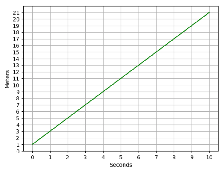
For this equation q(x) = 2x + 1, we can say the rate of change is 2. Generalizing, we have f(x) = mx + C, m is the rate of change.

We calculate the rate of change the same as the slope:

m = Δy/Δx

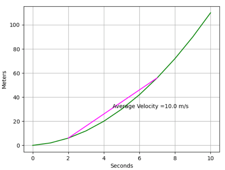
We can calculate the average rate of change between two points for a quadratic function like r(x) = x² + x.

It's possible to do it between the first and the last point of the function or in a period of time.

x = np.array(range(0, 11))
s = np.array([2,7])

x1 = s[0]
x2 = s[-1]
y1 = r(x1)
y2 = r(x2)
a = (y2 - y1)/(x2 - x1)

plt.xlabel('Seconds')
plt.ylabel('Meters')
plt.grid()
plt.plot(x,r(x), color='green')
plt.plot(s,r(s), color='magenta')
plt.annotate('Average Velocity =' + str(a) + ' m/s',((x2+x1)/2, (y2+y1)/2))
plt.show()

This plots the behavior of the function and average velocity:

Limits

In a quadratic equation, we have a bunch of points in the curve and we can plot like this:

def f(x):
  return x**2 + x

x = list(range(0,5))
x.append(4.25)
x.append(4.5)
x.append(4.75)
x.append(5)
x.append(5.25)
x.append(5.5)
x.append(5.75)
x = x + list(range(6,11))

y = [f(i) for i in x]

plt.xlabel('x')
plt.ylabel('f(x)')
plt.grid()
plt.plot(x,y, color='lightgrey', marker='o', markeredgecolor='green', markerfacecolor='green')
plt.show()

Generating this graph:

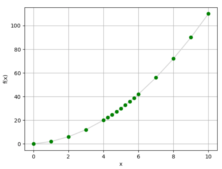
But we can still see gaps between points. And now we need to understand the concept of limits.

Not all functions are continuous. Take this function as an example:

g(x) = -(12/2x)², where x ≠ 0

x can't be 0 because any number divided by 0 is undefined.

def g(x):
  if x != 0:
    return -(12/(2 * x))**2

x = range(-20, 21)
y = [g(a) for a in x]

plt.xlabel('x')
plt.ylabel('g(x)')
plt.grid()
plt.plot(x,y, color='green')
plt.show()

Plotting g(x), we get this graph:

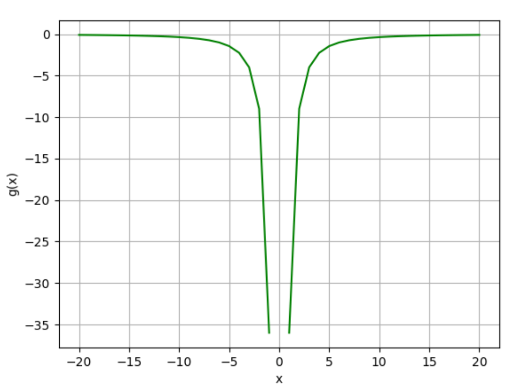
The function g(x) is non-continuous at x = 0

Limits can be applied to continuous functions like a(x) = x² + 1

When x is approaching 0, a(x) = 1.

That's because when x is slightly greater than 0 and slightly smaller than 0 (e.g. 0.000001 and -0.000001), the result will be slightly greater than 1 and slightly smaller than 1, respectively.

This is how we write it: when x approaches 0, the limit of a(x) is 1.

lim x->0 a(x) = 1

We can also apply this concept to non-continuous points. Take this function as an example: b(x) = -2x²/x, where x ≠ 0.

Let's plot it with Python

def b(x):
  if x != 0:
    return (-2*x**2) * 1/x

x = range(-10, 11)
y = [b(i) for i in x]

plt.xlabel('x')
plt.ylabel('b(x)')
plt.grid()
plt.plot(x,y, color='purple')
plt.show()

Here's what it looks like in a graph:

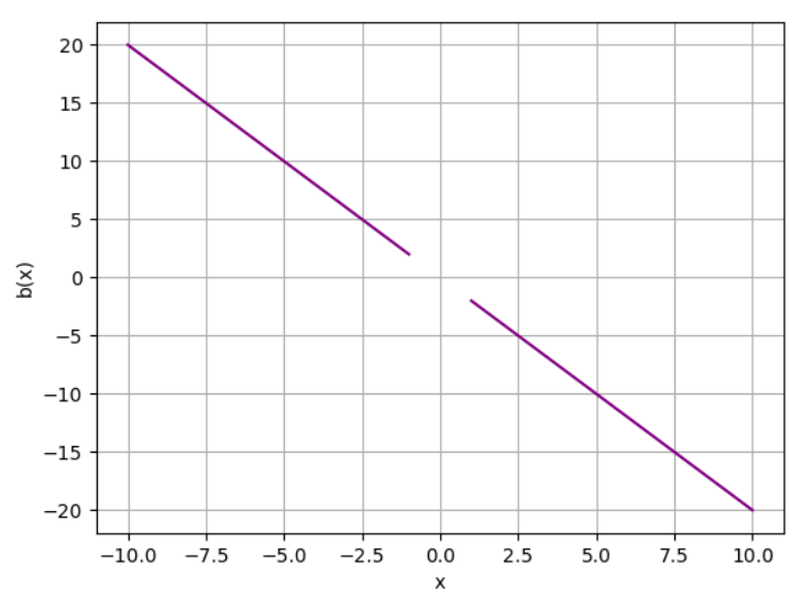
x approaching 0 from positive and negative sides equals 0

• lim x -> 0⁺ b(x) = 0
• lim x -> 0⁻ b(x) = 0

We can also approach infinite. Take this function: d(x) = 4 / (x - 25), where x ≠ 25

def d(x):
  if x != 25:
    return 4 / (x - 25)

x = list(range(-100, 24))
x.append(24.9)
x.append(25)
x.append(25.1)
x = x + list(range(26, 101))
y = [d(i) for i in x]

plt.xlabel('x')
plt.ylabel('d(x)')
plt.grid()
plt.plot(x,y, color='purple')
plt.show()

We plot this graph:

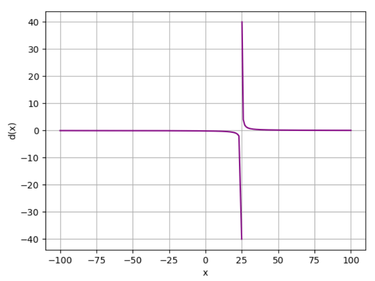
Approaching from negative and positive sides results in infinite.

• -♾️ when approaching from the negative side: lim x->25 d(x) = -♾️
• +♾️ when approaching from the positive side: lim x->25 d(x) = +♾️

We can use factorization when direct substitution doesn't work. Take this function as an example:

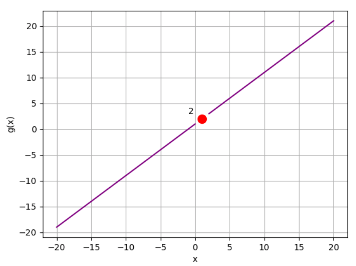
g(x) = (x² - 1) / (x - 1)

If we calculate the limit of x approaching 1, it won't work. The denominator can't be 0.

But if we use factorization, we can get an answer for this limit. Remember this generalization?

a² - b² = (a - b)(a + b)

We can use this rule for our g(x) function.

x² - 1 = (x - 1)(x + 1)
g(x) = (x - 1)(x + 1) / (x - 1)
g(x) = x + 1

Now we can calculate the limit of x approaching 1:

lim x->1 g(x) = x + 1
lim x->1 g(x) = 2

Let's plot the graph:

def g(x):
  if x != 1:
    return (x**2 - 1) / (x - 1)

x= range(-20, 21)
y =[g(i) for i in x]
zx = 1
zy = zx + 1

plt.xlabel('x')
plt.ylabel('g(x)')
plt.grid()
plt.plot(x, y, color='purple')
plt.plot(zx, zy, color='red', marker='o', markersize=10)
plt.annotate(str(zy), (zx, zy), xytext=(zx - 2, zy + 1))
plt.show()

Generating this graph:

We can use pretty much the same idea using rationalization.

Limits also have rules of operations: addition, subtraction, multiplication, division, etc.

Addition:

lim x->a (j(x) + l(x)) = lim x->a j(x) + lim x->a l(x)

Subtraction:

lim x->a (j(x) - l(x)) = lim x->a j(x) - lim x->a l(x)

Multiplication:

lim x->a (j(x) • l(x)) = lim x->a j(x) • lim x->a l(x)

Division:

lim x->a (j(x) / l(x)) = lim x->a j(x) / lim x->a l(x)

Exponentials and roots:

lim x->a (j(x))ⁿ = (lim x->a j(x))ⁿ

Differentiation and Derivatives

Calculating the slope m:

m = Δf(x) / Δx

or

m = (f(x₁) - f(x₀)) / (x₁ - x₀)

Making an adjustment with an increment for x, let's call it h, we have:

m = (f(x + h) - f(x)) / h

The shortest distance between x and x + h is when h is the smallest possible value, in other words, when h approaches 0.

f'(x) = lim h->0 (f(x + h) - f(x)) / h

We call it the derivative of the original function.

It's important because it provides valuable information about the behavior of a function at that specific point.

• Rate of change: how the function is changing at that specific point (crucial for understanding the dynamics of the system being modeled)
• Slope of the Tangent Line: useful for approximating the function locally by a linear function (simplify analysis and computation)
• Understanding Function Behavior: the sign of the derivative indicates whether the function is increasing or decreasing at that point
  • Find critical points: local maxima, minima, or saddle points
  • Important for optimization

Differentiability: be differentiable at every point; that is, you are able to calculate the derivative for every point on the function line

To be differentiable at a given point:

• The function must be continuous at that point.
• The tangent line at that point cannot be vertical
• The line must be smooth at that point (that is, it cannot take on a sudden change of direction at the point)

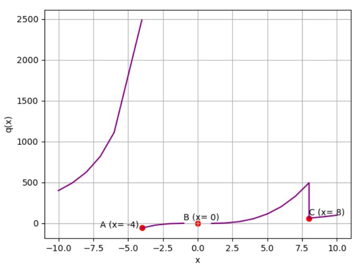
Take this function as an example:

q(x) = {
  40,000 / x², if x < -4,
  (x² - 2)·(x - 1), if x ≠ 0 and x ≥ -4 and x < 8,
  (x² - 2), if x ≠ 0 and x ≥ 8
}

Let's plot it with Python

def q(x):
  if x != 0:
    if x < -4:
      return 40000 / (x**2)
    elif x < 8:
      return (x**2 - 2) * x - 1
    else:
      return (x**2 - 2)

x = list(range(-10, -5))
x.append(-4.01)
x2 = list(range(-4,8))
x2.append(7.9999)
x2 = x2 + list(range(8,11))

y = [q(i) for i in x]
y2 = [q(i) for i in x2]

plt.xlabel('x')
plt.ylabel('q(x)')
plt.grid()
plt.plot(x,y, color='purple')
plt.plot(x2,y2, color='purple')
plt.scatter(-4,q(-4), c='red')
plt.annotate('A (x= -4)',(-5,q(-3.9)), xytext=(-7, q(-3.9)))
plt.scatter(0,0, c='red')
plt.annotate('B (x= 0)',(0,0), xytext=(-1, 40))
plt.scatter(8,q(8), c='red')
plt.annotate('C (x= 8)',(8,q(8)), xytext=(8, 100))
plt.show()

Here's the graph:

The points marked on this graph are non-differentiable:

• Point A is non-continuous - the limit from the negative side is infinity, but the limit from the positive side ≈ -57
• Point B is also non-continuous - the function is not defined at x = 0.
• Point C is defined and continuous, but the sharp change in direction makes it non-differentiable.

Derivative Rules

• f(x) = C, where C is a constant, then f'(x) = 0 (it's a horizontal lie)
• If f(x) = Cg(x), then f'(x) = Cg'(x)
• If f(x) = g(x) + h(x), then f'(x) = g'(x) + h'(x) (this also applies to subtraction)
• The power rule: f(x) = xⁿ ∴ f'(x) = nxⁿ⁻¹
• The product rule: d/dx[f(x)·g(x)] = f'(x)·g(x) + f(x)·g'(x)
• The quotient rule: r(x) = s(x) / t(x) ∴ r'(x) = (s'(x)·t(x) - s(x)·t'(x)) / [t(x)]²
• The chain rule: d/dx[O(i(x))] = o'(i(x))·i'(x)

Critical Points

Take this function:

k(x) = -10x² + 100x + 3

To determine the derivative function of the original function:

k'(x) = -20x + 100

And plotting with Python:

def k(x):
  return -10 * (x**2) + (100 * x)  + 3

def kd(x):
  return -20 * x + 100

x = list(range(0, 11))
y = [k(i) for i in x]
yd = [kd(i) for i in x]

plt.xlabel('x (time in seconds)')
plt.ylabel('k(x) (height in feet)')
plt.xticks(range(0,15, 1))
plt.yticks(range(-200, 500, 20))
plt.grid()
plt.plot(x,y, color='green')
plt.plot(x,yd, color='purple')
plt.show()

It generates these two functions in the graph:

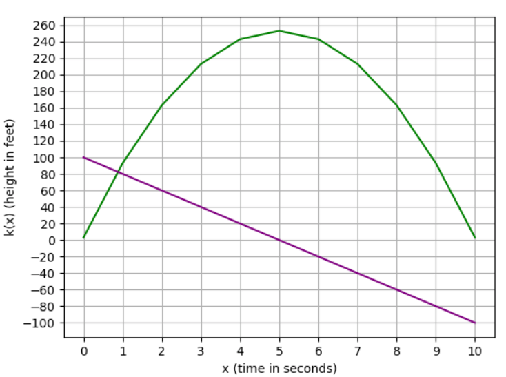
Some interpretations of this graph:

• The point where the derivative line crosses 0 on the y-axis is also the point where the function value stops increasing and starts decreasing. When the slope has a positive value, the function is increasing; and when the slope has a negative value, the function is decreasing.
• The tangent line (the slope in each point) is rotating clockwise throughout the graph.
• At the highest point, the tangent line would be perfectly horizontal, representing a slope of 0.

To illustrate the interpretation, we have three tangent lines: one when the function is increasing, one when the function is decreasing, and the other one when it's horizontal, in other words, when the slope is 0.

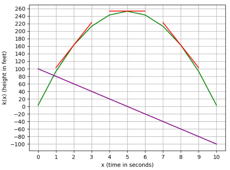
Critical points are represented when the derivative function crosses 0. It indicates that the function is changing direction.

Finding minima and maxima

k(x) = -10x² + 100x + 3
k'(x) = -20x + 100
-20x + 100 = 0
20x = 100
x = 100 / 20
x = 5

The derivative will be 0 when x is 5.

Second Order Derivatives

We can use second-order derivatives to determine if the critical point is minima or maxima.

k(x) = -10x² + 100x + 3
k'(x) = -20x + 100
k''(x) = -20

The second derivative has a constant value, so we know that the slope of the prime derivative is linear, and because it's a negative value, we know that it is decreasing.

When the derivative crosses 0, we know that the slope of the function is decreasing linearly, so the point at x = 0 must be a maximum point.

The same happens when finding a minimum point.

w(x) = x²+ 2x + 7
w'(x) = 2x + 2
w''(x) = 2

It's a positive constant, so it's increasing when crossing 0, therefore, it means this a minimum point.

Optimization is one of the applications of finding critical points.

Imagine a formula representing the expected number of subscriptions to Netflix:

s(x) = -5x + 100

In this case, s(x) is the number of subscriptions, and x is the monthly fee.

The monthly revenue can be calculated as the subscription volume times the monthly fee:

r(x) = s(x)·x
r(x) = -5x² + 100x

First, find the prime derivative:

r'(x) = -10x + 100

Then find the critical points (when r'(x) equals 0):

r'(x) = -10x + 100
0 = -10x + 100
10x = 100
x = 10

Finally checking if the critical point is a maximum or minimum point using the second-order derivative:

r'(x) = -10x + 100
r''(x) = -10
r''(10) = -10

A negative constant value in the second order derivative tells it's a maximum point. In other words, the maximum monthly fee for Netflix is 10.

Partial Derivatives

How do we calculate the derivate of multi-variables functions?

f(x, y) = x² + y²

We use partial derivatives:

• The derivative of f(x, y) with respect to x
• The derivative of f(x, y) with respect to y

Starting with the partial derivative with respect to x:

∂f(x, y) / ∂x
∂(x² + y²) / ∂x
∂x² / ∂x
2x

Because y doesn't depend on x, ∂y² / ∂x = 0

We get the same idea when calculating the partial derivative with respect to y:

∂f(x, y) / ∂y
∂(x² + y²) / ∂y
∂y² / ∂y
2y

We use partial derivatives to compute a gradient. A gradient is a way to find the analog of the slope for multi-dimensional surfaces.

You can find the minimum and maximum of curves using derivatives. In the same way, you can find the minimum and maximum of surfaces by following the gradient and finding the points where the gradient is zero in all directions.

For this function:

f(x, y) = x² + y²

We have

∂f(x, y) / ∂x = 2x
∂f(x, y) / ∂y = 2y

The gradient is a 2-dimensional vector:

grad(f(x, y)) = [2x, 2y]

We can use the concept of gradient in a minimization algorithm called the gradient descent method, where you take a guess, compute the gradient, take a small step in the direction of the gradient, and determine if it's close to 0 (the gradient will be 0 at the minimum).

The cost function provides a way to evaluate the performance of a model. Gradient descent is an optimization algorithm used to minimize the cost function. One type of cost function is the Mean Squared Error (MSE). Minimizing the cost function means

• Finding the model parameters that result in the smallest possible cost, indicating the best fit to the data.
• Lower values of the cost function indicate a model that better predicts the actual outcomes.

Resources

• Machine Learning Research
• Math for Machine Learning with Python

Twitter · Github