Linear Algebra Fundamentals
 Photo by MARIOLA GROBELSKA
This is the second part of the series Mathematics for Machine Learning with Python.
Vectors
What's a vector
A numeric element that has magnitude and direction.
- magnitude: distance
- direction: which way is headed
Let's see an example:
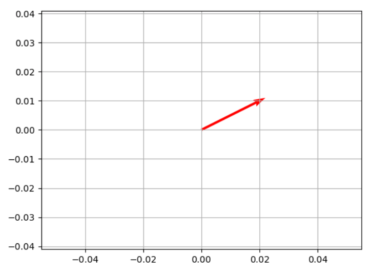
For this vector, we need to move 2 units in the x dimension and 1 unit in the y dimension. It's a way of saying the directions you need to follow to get to there from here.
import numpy as np
import matplotlib.pyplot as plt

vector = np.array([2, 1])
origin = [0], [0]
plt.axis('equal')
plt.grid()
plt.quiver(*origin, *vector, scale=10, color='r')
plt.show()
This will plot the vector in the graph:
Calculating Magnitude
We can use the Pythagorean theorem and calculate the square root of the sum of the squares.
v = √v₁² + v₂²
For our vector example: v = (2, 1), here's how I calculate it:
v = √2² + 1²
v = √4 + 1
v = √5 ≈ 2.24
In Python, we can use the math module:
import numpy as np
import math

vector = np.array([2, 1])
math.sqrt(vector[0]**2 + vector[1]**2) # 2.23606797749979
Calculating Direction
To calculate the direction (amplitude), we use trigonometry and get the angle of the vector by calculating the inverse tangent tan⁻¹.
tan(𝛉) = 1 / 2
𝛉 = tan⁻¹(0.5) ≈ 26.57°
We can confirm it by calculating it in Python
import math
import numpy as np

v = np.array([2,1])
vTan = v[1] / v[0] # 0.5
vAtan = math.atan(vTan)
math.degrees(vAtan) # 𝛉 = 26.56505117707799
Real Coordinate Spaces
A real coordinate space is all possible real-valued tuples and it's represented with this mathematical symbol
In linear algebra, we usually see this symbol showing also a number like this:
In this example, it's called the 2-dimensional real coordinate space, and it represents all possible real-valued 2-tuple. One example is this vector :
3 is the value for the horizontal axis and 4 for the vertical axis. We can also have different dimensions, like this:
Following the 2D, this is the 3D real coordinates space:
Both are members of the 3-tuple:
This could increase to an even bigger number. If this number is n, it would call it:
The n-dimensional real coordinate space.
Vector Addition
Let's add two vectors:
import numpy as np
import matplotlib.pyplot as plt

v = np.array([2, 1])
s = np.array([-3, 2])

vecs = np.array([v, s])
origin = [0], [0]
plt.axis('equal')
plt.grid()
plt.ticklabel_format(style='sci', axis='both', scilimits=(0,0))
plt.quiver(*origin, vecs[0, 0], vecs[0, 1], color=['r', 'b'], scale=10)
plt.quiver(*origin, vecs[1, 0], vecs[1, 1], color=['r', 'b'], scale=10)
plt.show()
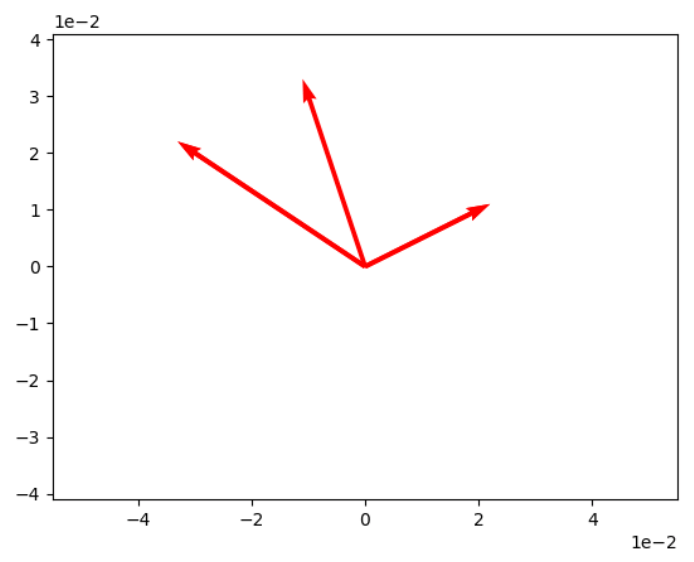
Let's calculate the sum of v and s, resulting in z:
Generate the new vector z with Python:
import numpy as np
import matplotlib.pyplot as plt

v = np.array([2, 1])
s = np.array([-3, 2])
z = v + s

vecs = np.array([v, s, z])
origin = [0], [0]
plt.axis('equal')
plt.grid()
plt.ticklabel_format(style='sci', axis='both', scilimits=(0,0))
plt.quiver(*origin, vecs[0, 0], vecs[0, 1], color=['r', 'b'], scale=10)
plt.quiver(*origin, vecs[1, 0], vecs[1, 1], color=['r', 'b'], scale=10)
plt.quiver(*origin, vecs[2, 0], vecs[2, 1], color=['r', 'b'], scale=10)
plt.show()
Here's the plot:
Vector Multiplication
We have 3 ways of performing vector multiplication:
- Scalar multiplication
- Dot product multiplication
- Cross product multiplication
Scalar multiplication is multiplying a vector by a single numeric value.
Let's multiply vector v by 2, resulting in a vector w.
v = (2, 1)
w = 2v
Here's how the multiplication is calculated:
w = (2·2, 2·1)
w = (4, 2)
In Python, we can use numpy to perform the vector multiplication
import numpy as np

v = np.array([2, 1])
w = 2 * v # [4 2]
The magnitude is 2 times longer. One way of thinking about this is that we scale it up by 3.
If we multiply the vector by -1, it won't change its magnitude, but it will change its direction.
The scalar division is the same idea:
import numpy as np

v = np.array([2, 1])
b = v / 2 # [1. 0.5]
In the dot production multiplication, we get the result of two vectors multiplication, in other words, the scalar product (a numeric value).
v·s = (v₁·s₁) + (v₂·s₂) ... + (vₙ·sₙ)
If v = (2, 1) and s = (-3, 2), here's how we calculate the scalar product:
v·s = (2·-3) + (1·2) = -6 + 2 = -4
In Python, we can use the dot method or @ to calculate the scalar product of two vectors.
# using .dot
v = np.array([2, 1])
s = np.array([-3, 2])
np.dot(v, s) # -4

# using @
v = np.array([2, 1])
s = np.array([-3, 2])
v @ s # -4
To get the vector product of multiplying two vectors, we need to calculate the cross product.
v = (2, 3, 1)
s = (1, 2, -2)
r = v·s = ? # vector product
We need to calculate the three components for the final vector:
r₁ = v₂s₃ - v₃s₂
r₂ = v₃s₁ - v₁s₃
r₃ = v₁s₂ - v₂s₁
Here's how we do the calculation in our example:
r = v·s = ((3·-2) - (1·-2), (1·1) - (2·-2), (2·2) - (3·1))
r = v·s = (-8, 5, 1)
In Python, we use the cross method:
p = np.array([2, 3, 1])
q = np.array([1, 2, -2])
r = np.cross(p, q) # [-8  5  1]
Matrices
What's a matrix
A matrix is an array of numbers that are arranged into rows and columns.
This is how you indicate each element in the matrix:
In Python, we can define the matrix as a 2-dimensional array:
import numpy as np

A = np.array([[1,2,3],
              [4,5,6]])
# [[1 2 3]
#  [4 5 6]]
To add two matrices of the same size together, just add the corresponding elements in each matrix:
Here's how we calculate it:
In Python, we can just sum the two matrices:
A = np.array([[1, 2, 3],
              [4, 5, 6]])

B = np.array([[6, 5, 4],
              [3, 2, 1]])

A + B
# [[7 7 7]
# [7 7 7]]
Subtraction of two matrices works the same way:
The negative of a matrix is just a matrix with the sign of each element reversed.
In Python, we can use the minus sign:
C = np.array([[-5, -3, -1],
              [1, 3, 5]])
C
# [[-5 -3 -1]
#  [ 1  3  5]]

-C
# [[ 5  3  1]
#  [-1 -3 -5]]
Matrix Transposition is when we switch the orientation of its rows and columns:
In Python, we have the T method:
A = np.array([[1, 2, 3],
              [4, 5, 6]])
A.T
# [[1 4]
#  [2 5]
#  [3 6]]
Matrix Multiplication
Scalar multiplication in matrices looks similar to scalar multiplication in vectors. To multiply a matrix by a scalar value, you just multiply each element by the scalar to produce a new matrix:
In Python, we simply perform the multiplication of two values:
A = np.array([[1,2,3],
              [4,5,6]])

2 * A
# [[ 2  4  6]
#  [ 8 10 12]]
To multiply two matrices, we need to calculate the dot product of rows and columns.
How to calculate this multiplication:
- First row from A times first column from B = First row, first column
- First row from A times second column from B = First row, second column
- Second row from A times first column from B = Second row, first column
- Second row from A times second column from B = Second row, second column
Resulting in these calculations:
(1·9) + (2·7) + (3·5) = 38
(1·8) + (2·6) + (3·4) = 32
(4·9) + (5·7) + (6·5) = 101
(4·8) + (5·6) + (6·4) = 86
Resulting in this matrix:
In Python, we can use the dot method or @:
import numpy as np

A = np.array([[1, 2, 3],
              [4, 5, 6]])

B = np.array([[9, 8],
              [7, 6],
              [5, 4]])

np.dot(A,B)
A @ B
# [[ 38  32]
#  [101  86]]
For matrix multiplication, we commutative law doesn't apply:
A = np.array([[2, 4],
              [6, 8]])

B = np.array([[1, 3],
              [5, 7]])

A @ B
# [[22 34]
#  [46 74]]

B @ A
# [[20 28]
#  [52 76]]
Identity matrices are matrices that have the value 1 in the diagonal positions and 0 in the rest of the other positions.
An example:
Multiplying a matrix by an identity matrix results in the same matrix. It's like multiplying by 1.
Matrix Division
Matrix division is basically multiplying it by the inverse of the matrix
How the inverse of a matrix is calculated? Using this equation:
Let's see it in action:
In Python, we can use the linalg.inv method:
import numpy as np

B = np.array([[6, 2],
              [1, 2]])

np.linalg.inv(B)
# [[ 0.2 -0.2]
#  [-0.1  0.6]]
Larger matrices than 2x2 are more complex to calculate the inverse, but it is calculated in the same way in Python:
B = np.array([[4, 2, 2],
              [6, 2, 4],
              [2, 2, 8]])

np.linalg.inv(B)
# [[-0.25   0.375 -0.125]
#  [ 1.25  -0.875  0.125]
#  [-0.25   0.125  0.125]]
With the calculation of the inverse, we can now calculate the multiplication of a matrix with an inverse of another matrix.
In Python, we can just invert the matrix and multiply by the inverse:
A = np.array([[1,2],
              [3,4]])

B = np.array([[6,2],
              [1,2]])

A @ np.linalg.inv(B)
# [[0.  1. ]
#  [0.2 1.8]]
Systems of Equations
We can write a system of equations in matrix form. Take a look a these equations:
We can write this in matrix form:
And we can write this in another way:
We know that A · X = B, which is the same as B ÷ A = X, which is the same as B · A⁻¹ = X.
The inverse of A is:
So:
The result of the matrix X is
In Python, we can confirm that:
A = np.array([[2, 4],
              [6, 2]])

B = np.array([[18],
              [34]])

X = np.linalg.inv(A) @ B
# [[5.]
#  [2.]]