Building a Linear Regression from Scratch with Python & Mathematics

2025-03-20

• 22 min read

time lapse and light streaks of vehicle on road

A couple of months ago, I wrote about building a neural network from scratch with only Python and Mathematics. Because I'm learning basic machine learning algorithms again, I decided to do a similar project and build a linear regression from scratch with Python and Mathematics.

Here are the topics of this article:

How to represent a linear model
The cost function: minimizing to optimize predictions
Gradient descent: parameters optimization
Vectorization: speed up the process
Multiple variable linear regression

Let's start.

Model Representation

The motivating example we'll use is a house price prediction problem. To make it very simple at the beginning, we'll use a dataset of only 2 examples with one feature (house size) and the target (price).

Size (1000 sqft)	Price (1000s of dollars)
1.0	300
2.0	500

As said above, we have the size as the only one feature (X) for this problem, and house prices as the target (Y), or the value we're trying to predict.

Here's how we can represent the data

x_train = np.array([1.0, 2.0])
y_train = np.array([300.0, 500.0])

print(f"x_train = {x_train}") # x_train = [1. 2.]
print(f"y_train = {y_train}") # y_train = [300. 500.]

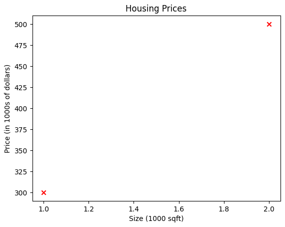
Using the scatter function from the matplotlib, we can plot the data into a graph:

plt.scatter(x_train, y_train, marker='x', c='r')
plt.title("Housing Prices")
plt.ylabel('Price (in 1000s of dollars)')
plt.xlabel('Size (1000 sqft)')
plt.show()

Here's what it looks like:

For a simple model like a linear regression, the model function is represented as

f(x) = wx + b

where $w$ is the model weight and $b$ is the bias.

A linear function with random Ws and Bs produces the model function. For a linear regression, the function is a line. The line is a function built by the learning algorithm (model). The function receives an input (features) and outputs a prediction (y-hat), the estimated value of y.

The idea of the model is to ask what the math formula for $f$ is.

Let's play around with $w$ and $b$ . To compute the model function for each training example, we have a function called compute_model. It receives the training data, a $w$ , and a $b$ of choice.

def compute_model(x, w, b):
    """
    Computes the prediction of a linear model
    Args:
      x (ndarray (m,)): Data, m examples
      w,b (scalar)    : model parameters
    Returns
      y (ndarray (m,)): target values
    """
    m = x.shape[0]
    f_wb = np.zeros(m)

    for i in range(m):
        f_wb[i] = w * x[i] + b

    return f_wb

m is the number of training examples in the dataset. For each training example, we compute the model function based on the representation illustrated before.

The returning value is all the predictions using the chosen $w$ and $b$ .

Let's say we have these parameters:

w = 100
b = 100

And we pass them to the compute_model function

output = compute_model(x_train, w, b)

The output is all the predictions based on those chosen parameters.

For w = 100 and b = 100, we can plot the results:

plt.plot(x_train, output, c='b', label='Prediction')
plt.scatter(x_train, y_train, marker='x', c='r', label='Actual Values')
plt.title('Housing Prices')
plt.ylabel('Price (in 1000s of dollars)')
plt.xlabel('Size (1000 sqft)')
plt.legend()
plt.show()

We have this plot:

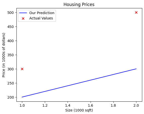
We can see that the chosen parameters don't result in a line that fits the data.

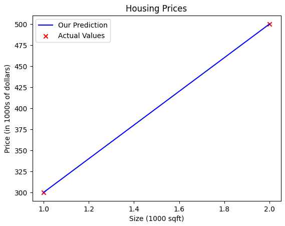
We can try different parameters until we find the perfect ones. Specifically for this dataset, we know that w = 200 and b = 100 are the parameters that fit the data perfectly.

w = 200
b = 100
output = compute_model(x_train, w, b)

plt.plot(x_train, output, c='b', label='Our Prediction')
plt.scatter(x_train, y_train, marker='x', c='r', label='Actual Values')
plt.title('Housing Prices')
plt.ylabel('Price (in 1000s of dollars)')
plt.xlabel('Size (1000 sqft)')
plt.legend()
plt.show()

This code plots this graph, and we can see how the model fits the data perfectly

With the perfect parameters, we can predict the price of a house based on its size. Let's say it is 1.2 in size (1000 sqft).

x_i = 1.2
cost_1200sqft = w * x_i + b

print(f"${cost_1200sqft:.0f} thousand dollars") # $340 thousand dollars

And this is our first prediction for a very simple linear regression.

Cost Function

To train the model to find the best parameters, we need to improve a certain metric. That way, the model knows it's learning. To measure this, we use the cost function. With this equation, we know how well the model's predictions match the dataset.

In our implementation, we'll be using the mean squared error cost function, which sums the square difference between the prediction and the real target over $m$ training examples.

J(w,b) = \frac{1}{2m} \sum\limits_{i = 0}^{m-1} (f_{w,b}(x^{(i)}) - y^{(i)})^2

where

f_{w,b}(x^{(i)}) = wx^{(i)} + b

For a given $W$ and $B$ , we measure the cost for all the training examples. The idea is to give this metric to the model and it will auto-adjust to find better parameters, which means choosing new parameters that minimize the cost. So the cost function is an important metric to measure how well the model is performing.

The implementation is quite simple:

def compute_cost(x, y, w, b):
    """
    Computes the cost function for linear regression.

    Args:
      x (ndarray (m,)): Data, m examples
      y (ndarray (m,)): target values
      w,b (scalar)    : model parameters

    Returns
        total_cost (float): The cost of using w,b as the parameters for linear regression
               to fit the data points in x and y
    """

    m = x.shape[0]
    cost_sum = 0

    for i in range(m):
        f_wb = w * x[i] + b
        cost = (f_wb - y[i]) ** 2
        cost_sum += cost

    total_cost = (1 / (2 * m)) * cost_sum

    return total_cost

We need to sum the cost for each training example using the chosen parameters $W$ and $B$ , so we iterate through the $m$ training examples, and for each, we need to compute the function $f$ and the cost, squaring the difference between $f$ and the actual target value.

After that, we just add it to the cost_sum. Compute all costs and sum. Then we just need to compute the total cost and return it from the function.

There's a faster approach for this function. The vectorization optimization.

def compute_cost(x, y, w, b):
    """
    Computes the cost function for linear regression.

    Args:
      x (ndarray (m,)): Data, m examples
      y (ndarray (m,)): target values
      w,b (scalar)    : model parameters

    Returns
        total_cost (float): The cost of using w,b as the parameters for linear regression
               to fit the data points in x and y
    """

    m = x.shape[0]
    cost_sum = 0
    f = w * x + b
    cost = (f - y) ** 2
    cost_sum = sum(cost)
    total_cost = (1 / (2 * m)) * cost_sum

    return total_cost

Instead of computing the cost for the training examples one by one, we do it all together in just one batch, with no loop required. This approach is much faster, especially for bigger datasets.

An illustration of the cost function helps build our intuition on how it works.

Let's say we have a new larger dataset:

x_train = np.array([1.0, 1.7, 2.0, 2.5, 3.0, 3.2])
y_train = np.array([250, 300, 480, 430, 630, 730])

We know the actual value and we can compute the prediction.

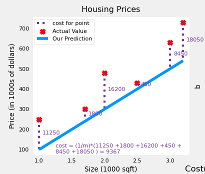
We calculate the difference between the actual value and the prediction, and we have the cost. The idea of the model is to find a line that fits the data better. So we optimize the parameters to form the line that will minimize the cost across all training examples.

Gradient Descent

The cost function was implemented before, and now we need to implement the algorithm that minimizes the cost so we can find the most optimized parameters $W$ and $B$ .

The algorithm we will use for this work is called gradient descent. The idea is pretty simple:

Have the linear function:

f_{w,b}(x^{(i)}) = wx^{(i)} + b

Compute the cost:

J(w,b) = \frac{1}{2m} \sum\limits_{i = 0}^{m-1} (f_{w,b}(x^{(i)}) - y^{(i)})^2

And here is the new part. We need to iterate a number of times (a hyperparameter we can pass to the model) until it converges. In each iteration, the model will update the parameters $W$ and $B$ .

This is how we update the parameters:

w = w - \alpha \frac{\partial J(w,b)}{\partial w}

b = b - \alpha \frac{\partial J(w,b)}{\partial b}

Let's break it down. $\alpha$ is the learning rate. It's a hyperparameter we use to control the step size to balance speed and stability when updating the parameters. Then we have the partial derivatives.

We need to compute the derivative of the cost function with respect to $W$ and then again with respect to $B$ . Here are the definitions:

\frac{\partial J(w,b)}{\partial w} = \frac{1}{m} \sum_{i = 0}^{m-1} (f_{w,b}(x^{(i)}) - y^{(i)})x^{(i)}

\frac{\partial J(w,b)}{\partial b} = \frac{1}{m} \sum_{i = 0}^{m-1} (f_{w,b}(x^{(i)}) - y^{(i)})

This measures how much the cost changes when $W$ and $B$ change by a small amount. This computation is also called gradient. Let's code that.

def compute_gradient(x, y, w, b):
    """
    Computes the gradient for linear regression
    Args:
      x (ndarray (m,)): Data, m examples
      y (ndarray (m,)): target values
      w,b (scalar)    : model parameters
    Returns
      dj_dw (scalar): The gradient of the cost w.r.t. the parameters w
      dj_db (scalar): The gradient of the cost w.r.t. the parameter b
     """

    m = x.shape[0]
    dj_dw = 0
    dj_db = 0

    for i in range(m):
        f_wb = w * x[i] + b
        dj_dw_i = (f_wb - y[i]) * x[i]
        dj_db_i = f_wb - y[i]
        dj_db += dj_db_i
        dj_dw += dj_dw_i

    dj_dw = dj_dw / m
    dj_db = dj_db / m

    return dj_dw, dj_db

The implementation is pretty simple and less scary than the math equations, especially if you don't have a good foundation in calculus. But it's basically partial derivatives in a loop.

The Cost x W graph looks like a curve and computing the gradients is computing the slope of the curve for a given cost and weight.

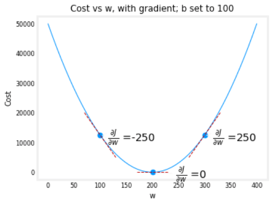
In this graph, we can see three gradients computed. The middle one is when the model converged and found the most optimized parameters for the given training dataset.

To put everything together, we will implement the gradient descent:

Loop through the number of iterations
Compute the gradients for $W$ and $B$
Update $W$ and $B$
Compute the cost using the cost function and store it in a history vector
With the end of the iterations, we have the final $W$ and $B$ , and then we can just return them

Here's the implementation

def gradient_descent(x, y, w_in, b_in, alpha, num_iters, cost_function, gradient_function):
    """
    Performs gradient descent to fit w,b. Updates w,b by taking
    num_iters gradient steps with learning rate alpha

    Args:
      x (ndarray (m,))  : Data, m examples
      y (ndarray (m,))  : target values
      w_in,b_in (scalar): initial values of model parameters
      alpha (float):     Learning rate
      num_iters (int):   number of iterations to run gradient descent
      cost_function:     function to call to produce cost
      gradient_function: function to call to produce gradient

    Returns:
      w (scalar): Updated value of parameter after running gradient descent
      b (scalar): Updated value of parameter after running gradient descent
      J_history (List): History of cost values
      p_history (list): History of parameters [w,b]
      """

    w = copy.deepcopy(w_in)
    J_history = []
    p_history = []
    b = b_in

    for i in range(num_iters):
        dj_dw, dj_db = gradient_function(x, y, w, b)

        b = b - alpha * dj_db
        w = w - alpha * dj_dw

        if i < 100000:
            J_history.append(cost_function(x, y, w, b))
            p_history.append([w, b])

        if i % math.ceil(num_iters / 10) == 0:
            print(f"Iteration {i:4}: Cost {J_history[-1]:0.2e} ",
                  f"dj_dw: {dj_dw: 0.3e}, dj_db: {dj_db: 0.3e}  ",
                  f"w: {w: 0.3e}, b:{b: 0.5e}")

    return w, b, J_history, p_history

Running it for the dataset, we have this output:

w_init = 0
b_init = 0
iterations = 10000
LR = 1.0e-2

w_final, b_final, J_hist, p_hist = gradient_descent(x_train ,y_train, w_init, b_init, LR,
                                                    iterations, compute_cost, compute_gradient)

print(f"(w,b) found by gradient descent: ({w_final:8.4f}, {b_final:8.4f})")

# Iteration    0: Cost 7.93e+04  dj_dw: -6.500e+02, dj_db: -4.000e+02   w:  6.500e+00, b: 4.00000e+00
# Iteration 1000: Cost 3.41e+00  dj_dw: -3.712e-01, dj_db:  6.007e-01   w:  1.949e+02, b: 1.08228e+02
# Iteration 2000: Cost 7.93e-01  dj_dw: -1.789e-01, dj_db:  2.895e-01   w:  1.975e+02, b: 1.03966e+02
# Iteration 3000: Cost 1.84e-01  dj_dw: -8.625e-02, dj_db:  1.396e-01   w:  1.988e+02, b: 1.01912e+02
# Iteration 4000: Cost 4.28e-02  dj_dw: -4.158e-02, dj_db:  6.727e-02   w:  1.994e+02, b: 1.00922e+02
# Iteration 5000: Cost 9.95e-03  dj_dw: -2.004e-02, dj_db:  3.243e-02   w:  1.997e+02, b: 1.00444e+02
# Iteration 6000: Cost 2.31e-03  dj_dw: -9.660e-03, dj_db:  1.563e-02   w:  1.999e+02, b: 1.00214e+02
# Iteration 7000: Cost 5.37e-04  dj_dw: -4.657e-03, dj_db:  7.535e-03   w:  1.999e+02, b: 1.00103e+02
# Iteration 8000: Cost 1.25e-04  dj_dw: -2.245e-03, dj_db:  3.632e-03   w:  2.000e+02, b: 1.00050e+02
# Iteration 9000: Cost 2.90e-05  dj_dw: -1.082e-03, dj_db:  1.751e-03   w:  2.000e+02, b: 1.00024e+02

# (w,b) found by gradient descent: (199.9929, 100.0116)

In the end, we have the most optimized parameters that minimize the cost function.

With more iterations, the cost decreases over time. We can see in the following illustration

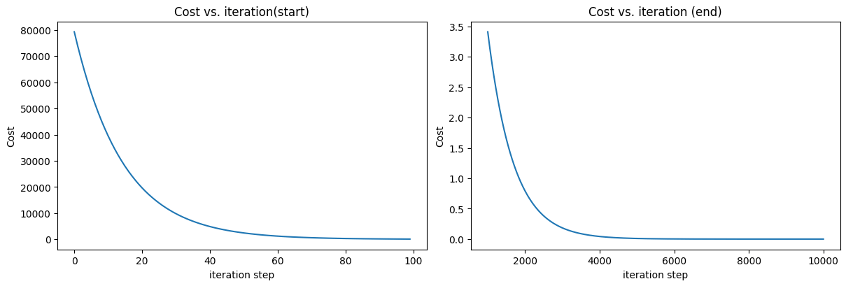
It's important to note that

The cost starts large and rapidly declines
The partial derivatives, dj_dw, and dj_db also get smaller, rapidly at first and then more slowly
Progress slows down, though the learning rate $\alpha$ remains fixed

With the optimal parameters $W$ and $B$ , we can predict the house prices for a new dataset.

print(f"1000 sqft house prediction {w_final*1.0 + b_final:0.1f} Thousand dollars")
print(f"1200 sqft house prediction {w_final*1.2 + b_final:0.1f} Thousand dollars")
print(f"2000 sqft house prediction {w_final*2.0 + b_final:0.1f} Thousand dollars")

This is the prediction output

1000 sqft house prediction 300.0 Thousand dollars
1200 sqft house prediction 340.0 Thousand dollars
2000 sqft house prediction 500.0 Thousand dollars

Before moving on to the next part of the implementation, we need to talk about the learning rate. The larger the $\alpha$ is, the faster gradient descent will converge to a solution. But, if it is too large, gradient descent will diverge.

w_init = 0
b_init = 0
iterations = 10
LR = 8.0e-1

w_final, b_final, J_hist, p_hist = gradient_descent(x_train ,y_train, w_init, b_init, LR,
                                                    iterations, compute_cost, compute_gradient)

Here's the iterations:

Iteration    0: Cost 2.58e+05  dj_dw: -6.500e+02, dj_db: -4.000e+02   w:  5.200e+02, b: 3.20000e+02
Iteration    1: Cost 7.82e+05  dj_dw:  1.130e+03, dj_db:  7.000e+02   w: -3.840e+02, b:-2.40000e+02
Iteration    2: Cost 2.37e+06  dj_dw: -1.970e+03, dj_db: -1.216e+03   w:  1.192e+03, b: 7.32800e+02
Iteration    3: Cost 7.19e+06  dj_dw:  3.429e+03, dj_db:  2.121e+03   w: -1.551e+03, b:-9.63840e+02
Iteration    4: Cost 2.18e+07  dj_dw: -5.974e+03, dj_db: -3.691e+03   w:  3.228e+03, b: 1.98886e+03
Iteration    5: Cost 6.62e+07  dj_dw:  1.040e+04, dj_db:  6.431e+03   w: -5.095e+03, b:-3.15579e+03
Iteration    6: Cost 2.01e+08  dj_dw: -1.812e+04, dj_db: -1.120e+04   w:  9.402e+03, b: 5.80237e+03
Iteration    7: Cost 6.09e+08  dj_dw:  3.156e+04, dj_db:  1.950e+04   w: -1.584e+04, b:-9.80139e+03
Iteration    8: Cost 1.85e+09  dj_dw: -5.496e+04, dj_db: -3.397e+04   w:  2.813e+04, b: 1.73730e+04
Iteration    9: Cost 5.60e+09  dj_dw:  9.572e+04, dj_db:  5.916e+04   w: -4.845e+04, b:-2.99567e+04

$W$ and $B$ are bouncing back and forth between positive and negative with the absolute value increasing with each iteration.

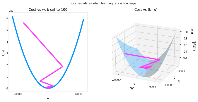
The learning rate is a hyperparameter that we need to find the optimal value for the dataset so the model can learn properly without diverging.

Small alpha: small baby steps in the gradient descent when updating the weight. slow to converge
Big alpha: large steps and the cost function can not reach the most optimized weight
Range of values: 0.001, 0.003, 0.01, 0.03, 0.1, 0.3, 1

It's important to check gradient descent's convergence

Make sure gradient descent is working by seeing the cost getting minimized with more iterations (learning curve)
When the curve gets flattened, gradient descent converges and stops learning
If the cost $J$ increases with more iterations, it usually means the learning rate $\alpha$ was chosen poorly, it can be too large, or a bug in the code

Multiple Variable Linear Regression

To implement a linear regression for a multiple variable dataset, we need to scale the dataset. Rather than having only the house size, we'll have other features like the number of bedrooms, number of floors, and age of the home. We can use all these features to predict the house price with a multiple variable linear regression.

| Size (sqft) | Number of Bedrooms | Number of floors | Age of Home | Price (1000s dollars) |
| ----------- | ------------------ | ---------------- | ----------- | --------------------- |
| 2104        | 5                  | 1                | 45          | 460                   |
| 1416        | 3                  | 2                | 40          | 232                   |
| 852         | 2                  | 1                | 35          | 178                   |

Here's the Python version for this dataset:

X_train = np.array([[2104, 5, 1, 45], [1416, 3, 2, 40], [852, 2, 1, 35]])
y_train = np.array([460, 232, 178])

For the training features $X$ , we have $m$ training examples and $n$ features. $X$ is a matrix with dimensions ( $m$ , $n$ ) ( $m$ rows, $n$ columns). Here's the matrix representation:

\begin{equation}\begin{pmatrix} x^{(0)}_0 & x^{(0)}_1 & \cdots & x^{(0)}_{n-1} \\ x^{(1)}_0 & x^{(1)}_1 & \cdots & x^{(1)}_{n-1} \\ \cdots \\ x^{(m-1)}_0 & x^{(m-1)}_1 & \cdots & x^{(m-1)}_{n-1} \end{pmatrix}\end{equation}

In terms of parameters, they will be a bit different. $B$ will still be a scalar value. But the $W$ will be a vector of $n$ values where each weight is there for each feature in the data set. ( $n$ features, $n$ is 4 for this dataset).

\begin{equation} W = \begin{pmatrix} w_0 \\ w_1 \\ \cdots \\ w_{n-1} \end{pmatrix}\end{equation}

This is how we represent the initial values for weight and bias

b_init = 785.1811367994083
w_init = np.array([0.39133535, 18.75376741, -53.36032453, -26.42131618])

Now that we have the training data and the parameters, we can define the linear model.

A previous model had only one feature so it needed only one weight. Now that we handle multiple variables, the model needs multiple parameters.

f_{w,b}(x) = w_0x_0 + w_1x_1 +... + w_{n-1}x_{n-1} + b

It's also possible to use the vector notion:

f_{w,b}(X) = W \cdot X

Let's go to our implementation. First, we'll compute the house price prediction for a single example using the initial parameters.

def predict_single_loop(x, w, b):
    """
    single predict using linear regression

    Args:
      x (ndarray): Shape (n,) example with multiple features
      w (ndarray): Shape (n,) model parameters
      b (scalar):  model parameter

    Returns:
      p (scalar):  prediction
    """
    n = x.shape[0]
    p = 0

    for i in range(n):
        p_i = x[i] * w[i]
        p = p + p_i

    p = p + b

    return p

For fixed parameters $w$ and $b$ , we loop through all the features for a single example and compute the prediction following the linear model definition. Because $b$ is a scalar value, we can add it later to the prediction and return it.

x_vec = X_train[0,:]
f_wb = predict_single_loop(x_vec, w_init, b_init)
print(f"f_wb prediction: {f_wb}")
# f_wb prediction: 459.9999976194083

As we did before, there's a much faster way to compute the linear model compared to the loop. And that's vectorization using the vector dot product.

def predict(x, w, b):
    """
    single predict using linear regression
    Args:
      x (ndarray): Shape (n,) example with multiple features
      w (ndarray): Shape (n,) model parameters
      b (scalar):             model parameter

    Returns:
      p (scalar):  prediction
    """
    return np.dot(x, w) + b

Let's test it

x_vec = X_train[0,:]
f_wb = predict(x_vec,w_init, b_init)
print(f"f_wb prediction: {f_wb}")
# f_wb prediction: 459.9999976194083

We can now make the model predict the house prices for multiple variables. The next step is to make it learn. And when I say “learn”, I mean computing the cost, computing the gradients, and updating the weights to find the optimal parameters.

So the next step is to compute the cost function for multiple variables.

Just to recap, the cost equation is the following

J(w,b) = \frac{1}{2m} \sum\limits_{i = 0}^{m-1} (f_{w,b}(x^{(i)}) - y^{(i)})^2

Before, we only had one feature. Now, we have multiple features in the dataset. Similar to what we did above using the dot product, we can use the same approach to compute the cost function.

def compute_cost(X, y, w, b):
    """
    compute cost
    Args:
      X (ndarray (m,n)): Data, m examples with n features
      y (ndarray (m,)) : target values
      w (ndarray (n,)) : model parameters
      b (scalar)       : model parameter

    Returns:
      cost (scalar): cost
    """
    m = X.shape[0]
    cost = 0.0

    for i in range(m):
        f_wb_i = np.dot(X[i], w) + b
        cost = cost + (f_wb_i - y[i])**2

    cost = cost / (2 * m)

    return cost

We need to compute the $y$ so we can calculate the cost value. We use the dot product to compute the prediction with the multiple variables and loop through all the training examples.

Let's test it:

cost = compute_cost(X_train, y_train, w_init, b_init)
print(f'Cost at optimal w : {cost}')
# Cost at optimal w : 1.5578904330213735e-12

Cool! We now have the cost function implemented. But before moving on to the next step, let's optimize it. Remember that we can use vectorization to optimize loops. Instead of looping through all the training examples, sum everything together to compute the cost.

def compute_cost(X, y, w, b):
    """
    compute cost
    Args:
      X (ndarray (m,n)): Data, m examples with n features
      y (ndarray (m,)) : target values
      w (ndarray (n,)) : model parameters
      b (scalar)       : model parameter

    Returns:
      cost (scalar): cost
    """
    m, _ = X.shape
    f_wb = np.dot(X, w) + b
    cost = np.sum((f_wb - y)**2) / (2 * m)

    return cost

The test should output the same cost value:

cost = compute_cost(X_train, y_train, w_init, b_init)
print(f'Cost at optimal w : {cost}')
# Cost at optimal w : 1.5578904330213735e-12

The next two remaining parts are the computation of gradients and the full gradient descent algorithm.

We need to compute the gradient for both $w$ and $b$ . The implementation looks similar to the one implemented before for a single feature linear regression. The difference is that, instead of having only one feature, we need to loop through all features to compute the gradient for $w$ .

def compute_gradient(X, y, w, b):
    """
    Computes the gradient for linear regression
    Args:
      X (ndarray (m,n)): Data, m examples with n features
      y (ndarray (m,)) : target values
      w (ndarray (n,)) : model parameters
      b (scalar)       : model parameter

    Returns:
      dj_dw (ndarray (n,)): The gradient of the cost w.r.t. the parameters w.
      dj_db (scalar):       The gradient of the cost w.r.t. the parameter b.
    """
    m, n = X.shape
    dj_dw = np.zeros((n,))
    dj_db = 0.

    for i in range(m):
        error = (np.dot(X[i], w) + b) - y[i]

        for j in range(n):
            dj_dw[j] = dj_dw[j] + error * X[i, j]

        dj_db = dj_db + error

    dj_dw = dj_dw / m
    dj_db = dj_db / m

    return dj_db, dj_dw

The gradient for $w$ is a vector because we are dealing with multiple variables, so each feature needs its own weight parameter. Bias is still a scalar value.

dj_db, dj_dw = compute_gradient(X_train, y_train, w_init, b_init)
print(f'dj_db: {dj_db}')
print(f'dj_dw: \n {dj_dw}')

# dj_db: -1.6739251122999121e-06
# dj_dw: [-2.73e-03 -6.27e-06 -2.22e-06 -6.92e-05]

We can vectorize this implementation too.

def compute_gradient(X, y, w, b):
    """
    Computes the gradient for linear regression
    Args:
      X (ndarray (m,n)): Data, m examples with n features
      y (ndarray (m,)) : target values
      w (ndarray (n,)) : model parameters
      b (scalar)       : model parameter

    Returns:
      dj_dw (ndarray (n,)): The gradient of the cost w.r.t. the parameters w.
      dj_db (scalar):       The gradient of the cost w.r.t. the parameter b.
    """
    m, n = X.shape
    error = ((np.dot(X, w) + b) - y)
    dj_db = np.sum(error) / m
    dj_dw = (np.dot(X_train.T, error.reshape(-1, 1)) / m).flatten()
    return dj_db, dj_dw

Here's the vectorization implementation:

Instead of computing the error for each training example, we compute all the errors in one batch
Instead of computing the gradient for $b$ for each training example, compute the value in one batch
Instead of computing the gradient for $w$ for each training example and each feature, compute it in one batch

Testing it again, we have the same values, as expected:

dj_db, dj_dw = compute_gradient(X_train, y_train, w_init, b_init)
print(f'dj_db: {dj_db}')
print(f'dj_dw: \n {dj_dw}')

# dj_db: -1.6739251122999121e-06
# dj_dw: [-2.73e-03 -6.27e-06 -2.22e-06 -6.92e-05]

The last part is to put everything together and implement the gradient descent algorithm. We did that already before and the implementation is quite similar. The only real difference is the fact that $X$ is a dataset of $m$ training examples and $n$ features.

def gradient_descent(X, y, w_in, b_in, cost_function, gradient_function, alpha, num_iters):
    """
    Performs batch gradient descent to learn theta. Updates theta by taking
    num_iters gradient steps with learning rate alpha

    Args:
      X (ndarray (m,n))   : Data, m examples with n features
      y (ndarray (m,))    : target values
      w_in (ndarray (n,)) : initial model parameters
      b_in (scalar)       : initial model parameter
      cost_function       : function to compute cost
      gradient_function   : function to compute the gradient
      alpha (float)       : Learning rate
      num_iters (int)     : number of iterations to run gradient descent

    Returns:
      w (ndarray (n,)) : Updated values of parameters
      b (scalar)       : Updated value of parameter
      """

    J_history = []
    w = copy.deepcopy(w_in)
    b = b_in

    for i in range(num_iters):
        dj_db, dj_dw = gradient_function(X, y, w, b)
        w = w - alpha * dj_dw
        b = b - alpha * dj_db
        J_history.append(cost_function(X, y, w, b))

        if i % math.ceil(num_iters / 10) == 0:
            print(f"Iteration {i:4d}: Cost {J_history[-1]:8.2f}")

    return w, b, J_history

To test it, we need to run the gradient descent with the dataset and check the cost in each iteration:

initial_w = np.zeros_like(w_init)
initial_b = 0.
iterations = 1000
alpha = 5.0e-7

w_final, b_final, J_hist = gradient_descent(X_train, y_train, initial_w, initial_b,
                                            compute_cost, compute_gradient,
                                            alpha, iterations)

Here are the computed costs over time:

Iteration    0: Cost  2529.46
Iteration  100: Cost   695.99
Iteration  200: Cost   694.92
Iteration  300: Cost   693.86
Iteration  400: Cost   692.81
Iteration  500: Cost   691.77
Iteration  600: Cost   690.73
Iteration  700: Cost   689.71
Iteration  800: Cost   688.70
Iteration  900: Cost   687.69

At the end of the algorithm, we find the optimal parameters:

print(f"b,w found by gradient descent: {b_final:0.2f},{w_final}")
# b, w found by gradient descent: -0.00, [ 0.2   0.   -0.01 -0.07]

Now we can compare the real values with the predicted ones:

m, _ = X_train.shape

for i in range(m):
    print(f"prediction: {np.dot(X_train[i], w_final) + b_final:0.2f}, target value: {y_train[i]}")

Here are the comparisons:

prediction: 426.19, target value: 460
prediction: 286.17, target value: 232
prediction: 171.47, target value: 178

Resources

Hey! You may like this newsletter if you're enjoying this blog. ❤

✖

Twitter · Github