Building A Neural Network from Scratch with Mathematics and Python

2024-11-17

• 20 min read

I've been studying machine learning and AI for quite some time now but neural networks caught my attention because of their nature of modeling, understanding, and learning abstract, complex, and unstructured data. It's been 2 or 3 months that I've been reading books, doing courses, and coding neural nets but I was eager to officially write down all my notes and learnings.

This post aims to be a comprehensive article about neural networks, how mathematics works, and provide an implementation from scratch in Python and Numpy, without any other framework, like Tensorflow or Pytorch.

Here are the following topics I'm going to cover in this post:

Introduction of Neural Networks
Mathematics of Neural Networks
Digit Recognizer Problem & Python Implementation

Introduction of Neural Networks

A neural network is a combination of the input, layers, neurons, and the output.

A simple neural network will receive data as input, process the data in the hidden layers through linear combinations and activation functions, and result in an output. The output can be a label — for binary or multiclass classification problems — or a continuous value if we are working with a regression problem.

For a simple neural network, let's say a 2-layer neural network, it has an input layer, a hidden layer where we do our first linear combination together with the application of an activation function, and then we have our second layer, also called, in this case, the output layer, where we also have a linear combination and then apply a different activation function to classify or predict an estimate, depending on the problem.

For the input layer, we use the symbol $X$ and this is a matrix of all features and training examples. The features are usually the columns and the rows are all training examples. It's commonly used m as the number of rows (training examples) and n as the number of columns (features).

And then we have the hidden layer. The neural network makes a bunch of connections between the input and the hidden layers.

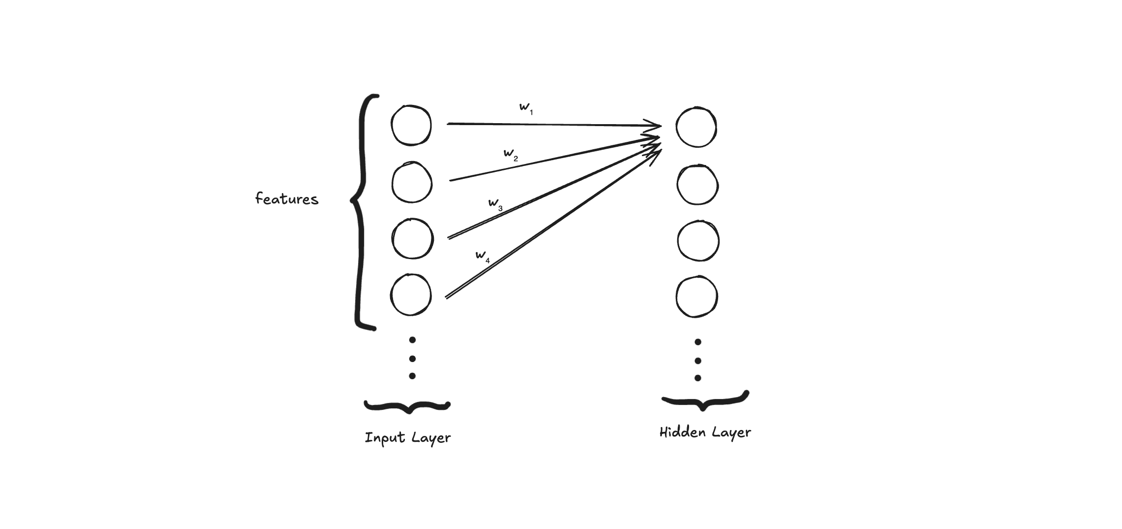
Each neuron, also called a hidden unit, will do two main things:

Compute a linear combination (input, weight, and bias)
Compute the activation function for this linear combination

The linear combination is basically the input data times a weight $w$ plus a bias term $b$ . Both $w$ and $b$ are parameters that the neural network will use in the learning process.

\begin{equation}z = w x + b\end{equation}

In linear algebra, linear combinations are usually symbolized with a $z$ .

After the linear combination, we need to apply an activation function. It's a non-linear function to add complexity to the model. Different types of functions can be applied here: sigmoid, tanh, ReLU, etc.

Activation functions allow the network to learn and represent complex patterns by introducing non-linearities, enabling it to approximate complex functions. It also helps the neural network to generalize and learn abstract features. It also allows gradients to be meaningful, enabling efficient learning.

The output of this first hidden layer is represented by the symbol $A$ . With many layers in the neural network, we need to name them with the layer number, like ${A^{[1]}}$ , ${A^{[2]}}$ , ${A^{[3]}}$ , etc.

The output layer has a similar structure to the hidden layer. It computes the linear combination and the activation function. The difference is that the input for this layer is ${A^{[1]}}$ , the output of the first layer and we use a different activation function to compute the prediction. For example, It can be a linear function for a regression problem, a sigmoid function for a binary classification, or softmax for a multiclass classification problem.

With the prediction, we can now measure how well our neural network model’s predictions align with the actual target values. In other words, we compute a loss function.

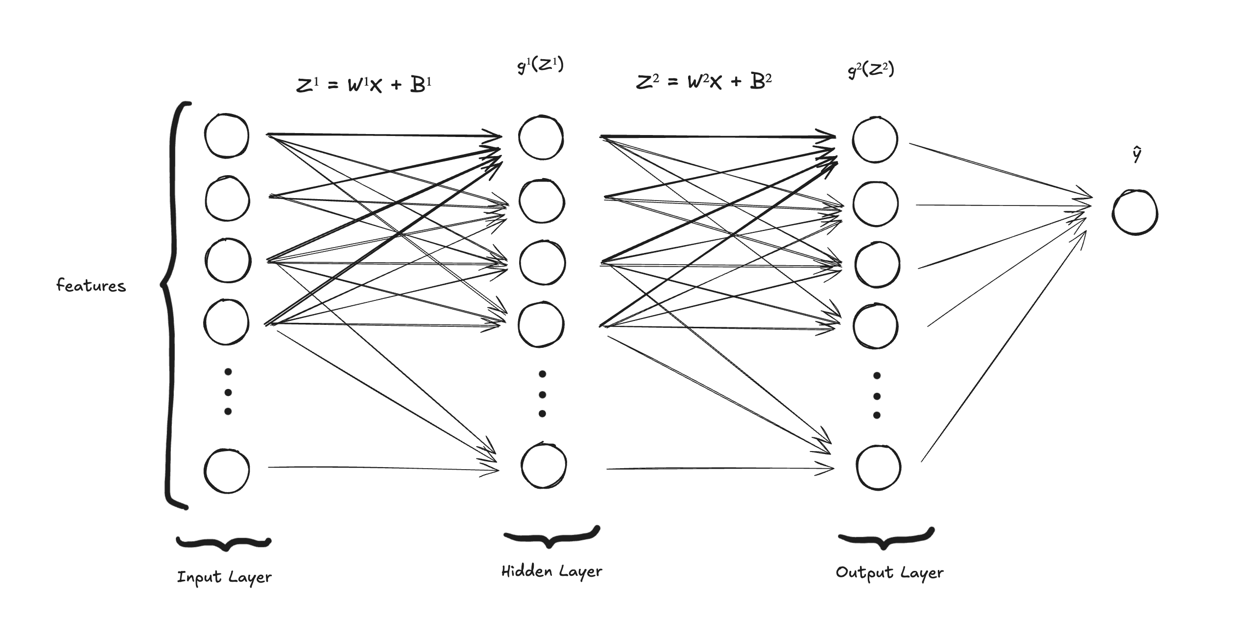
This whole process from input to the hidden layer to the output layer and finally resulting in a prediction is called forward propagation.

If we only compute the forward propagation, we only have one estimate and the neural network is not really learning anything. It just calculated one prediction. So we need a way to make the neural network learn. This learning process is a combination of backpropagation and an optimization algorithm (e.g. gradient descent).

The backpropagation process starts from the output and goes all the way to the starting point of the neural network. The idea is to compute derivatives of the loss function with respect to parameters like weights and biases for the different layers. Because the loss function measures how the model is performing, we want to minimize it as much as possible so it can perform better and better. With these calculations, we know the rate of change between the loss function and the parameter (weight and bias) so we can update the weights and biases with the goal of minimizing the loss function, enabling the neural network to learn and perform better.

We can repeat this back-and-forward process many times, updating the parameters (weights and biases) to minimize the loss function. In other words, we make the neural network learn better in each iteration.

Mathematics of Neural Networks

Let's now build up the maths for the neural network. We'll start with the forward propagation and do backpropagation right after.

We have a matrix as the input layer and we'll use it as the input for the first hidden layer. The symbol we use here is $X$ .

To compute the hidden layer, we first need to compute the linear combination:

\begin{equation}Z^{[1]} = W^{[1]} X + B^{[1]}\end{equation}

We call a linear combination as $Z$ , or in this case ${Z^{[1]}}$ because it's the linear combination of the first layer.

Then we need to apply the activation function, symbolized by ${g^{[1]}}$ , resulting in the output of the first layer: ${A^{[1]}}$ .

\begin{equation}A^{[1]} = g^{[1]}(Z^{[1]})\end{equation}

In the following section, we'll talk about the classification problem we'll apply all this theory and the activation function we'll use is one called Rectified Linear Unit (ReLU) which is a very simple function and easy to implement and derive.

\begin{equation}f(Z) = max(Z, 0)\end{equation}

In words, the ReLU function outputs:

z if z > 0
0 if z ≤ 0.

All of this is for the first layer. The second layer is pretty much the same idea but we annotate the symbols with 2 to specify we are talking about the second one.

\begin{equation}Z^{[2]} = W^{[2]} A^{[1]} + B^{[2]}\end{equation}

\begin{equation}A^{[2]} = g(Z^{[2]})\end{equation}

For the second activation function, we'll be using a different one than ReLU because we want to compute the probability of multi-label classification. The function is called softmax.

\begin{equation}softmax(x_i) = \frac{e^{x_i}}{sum_{j=1}^{k} e^{x_j}}\end{equation}

The output of this function is the probability of all input values. The predicted label will be the class with a higher probability score. All the possible labels have a probability and if sum all of them, we get 1 (or 100%).

After finishing the forward propagation, we need to compute the backpropagation. Mathematically, this step is the real challenge, especially if you have a hard time with maths and calculus. The entire backpropagation is about derivatives.

But why derivatives? Because we want to compute something called gradients, and then implement an algorithm called gradient descent as the optimizer of our neural network.

Until now, what we did was to compute an output, a prediction. In this case, the probability of different classes or labels. But if we do it just one time, the neural network is not learning.

The learning process is about “how much the loss function minimizes if we change the model parameters?” and keep changing them until it's “enough”. In other words, we want to understand how much the loss function will change if we change the $w$ and $b$ parameters. We update them and repeat the process so for each iteration, the neural network is learning more and more patterns and performing better over time.

This concept of “rate of change” of the loss function with respect to parameter $w$ or parameter $b$ is basically a derivative.

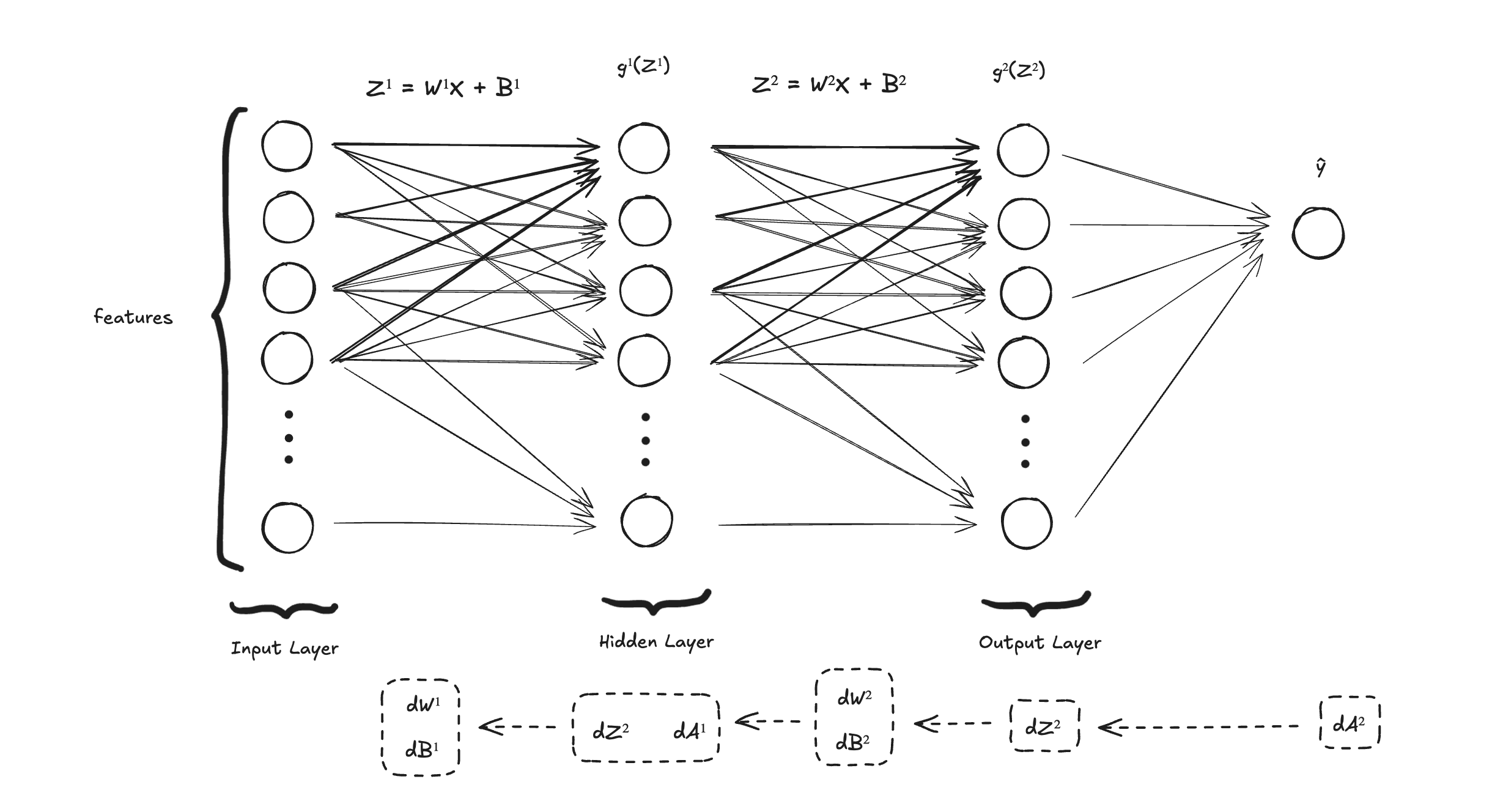
We compute the gradients from the end of the neural network all the way to the beginning of it. Here are all the steps we need to do then:

$\frac{dL}{dz^{[2]}} = dz^{[2]} =$ derivative of the loss function with respect to $z^{[2]}$

$\frac{dL}{dw^{[2]}} = dw^{[2]} =$ derivative of the loss function with respect to $w^{[2]}$

$\frac{dL}{db^{[2]}} = db^{[2]} =$ derivative of the loss function with respect to $b^{[2]}$

$\frac{dL}{dz^{[1]}} = dz^{[1]} =$ derivative of the loss function with respect to $z^{[1]}$

$\frac{dL}{dw^{[1]}} = dw^{[1]} =$ derivative of the loss function with respect to $w^{[1]}$

$\frac{dL}{db^{[1]}} = db^{[1]} =$ derivative of the loss function with respect to $b^{[1]}$

Let's compute that.

To compute ${dz^{[2]}}$ , we need to do the derivative of the loss function and ${dz^{[2]}}$ . This is basically the chain rule: To compute $\frac{dL}{dz^{[2]}} = \frac{dL}{da} \cdot \frac{da}{dz^{[2]}}$ , which is calculated as ${a}^{[2]} - y$ , where ${a}^{[2]}$ is the predicted value and $y$ is the real label.

For the weight in the second layer, we compute this derivative: $\frac{dL}{dw^{[2]}} = {dw^{[2]}} = \frac{dL}{dz^{[2]}} \cdot \frac{dz^{[2]}}{dw^{[2]}} = {({a}^{[2]} - y)} \cdot {a^{[1]}}^T$ .

The computation for the bias is similar to the weight but we compute the derivative of the loss function with respect to the bias in the second layer: $\frac{dL}{db^{[2]}} = {db^{[2]}} = \frac{dL}{dz^{[2]}} \cdot \frac{dz^{[2]}}{db^{[2]}} = {dz^{[2]}}$ .

$\frac{dL}{dz^{[1]}} = {dz^{[1]}}$ : the derivative of the loss function with respect to $z^{[1]}$ is a bigger chain rule: $\frac{dL}{dz^{[2]}} \cdot \frac{dz^{[2]}}{da^{[1]}} \cdot \frac{da^{[1]}}{dz^{[1]}}$ , producing ${w^{[2]}}^T \cdot {dz^{[2]}} \cdot g\'(z^{[1]})$

$g\'(z^{[1]})$ is the derivative of the loss function with respect to the activation function $g$ . In the example of this post, we need to do the derivative of the ReLU activation function.

Because a ReLU function is $z$ if $z > 0$ and 0 if $z \le 0$ , the derivative of it is 1 if $z > 0$ and 0 if $z \le 0$ . In the practice example, we'll see how this is very simple to implement in Python and Numpy.

The derivative of $\frac{dL}{dw^{[1]}} = {dw^{[1]}}$ is $\frac{dL}{dz^{[2]}} \cdot \frac{dz^{[2]}}{da^{[1]}} \cdot \frac{da^{[1]}}{dz^{[1]}} \cdot \frac{dz^{[1]}}{dw^{[1]}}$ , producing $dz^{[1]} \cdot x^T$

The derivative of $\frac{dL}{db^{[1]}} = {db^{[1]}}$ is $\frac{dL}{dz^{[2]}} \cdot \frac{dz^{[2]}}{da^{[1]}} \cdot \frac{da^{[1]}}{dz^{[1]}} \cdot \frac{dz^{[1]}}{db^{[1]}}$ , producing $dz^{[1]}$

That's so interestingly intuitive because if we see the chain rule, we can see the backpropagation in this computation from $z^{[2]}$ to the first parameters $w^{[1]}$ and $b^{[1]}$ .

So here are all the derivatives together:

\begin{equation}\frac{dL}{dz^{[2]}} = dz^{[2]} = {a}^{[2]} - y\end{equation}

\begin{equation}\frac{dL}{dw^{[2]}} = dw^{[2]} = {({a}^{[2]} - y)} \cdot {a^{[1]}}^T\end{equation}

\begin{equation}\frac{dL}{db^{[2]}} = db^{[2]} = dz^{[2]}\end{equation}

\begin{equation}\frac{dL}{dz^{[1]}} = dz^{[1]} = {w^{[2]}}^T \cdot {dz^{[2]}} \cdot g\'(z^{[1]})\end{equation}

\begin{equation}\frac{dL}{dw^{[1]}} = dw^{[1]} = dz^{[1]} \cdot x^T\end{equation}

\begin{equation}\frac{dL}{db^{[1]}} = db^{[1]} = dz^{[1]}\end{equation}

But this is a computation for only one training example. We need to do this for all the training examples in the dataset. Rather than implementing a loop, we can use a much faster operation called vectorization. In this process, we compute operations between matrices.

So, instead of computing for just one value $z$ , we do it for all the training examples. We symbolize it with $Z$ (capital Z). Here are all the derivatives using vectorization:

\begin{equation}dZ^{[2]} = {A}^{[2]} - Y\end{equation}

\begin{equation}dW^{[2]} = \frac{1}{m} \cdot {dZ}^{[2]} \cdot {A^{[1]}}^T\end{equation}

\begin{equation}dB^{[2]} = \frac{1}{m} \cdot \sum_{i=1}^m dZ^{[2]}\end{equation}

\begin{equation}dZ^{[1]} = {W^{[2]}}^T \cdot {dZ^{[2]}} \cdot g\'(Z^{[1]})\end{equation}

\begin{equation}dW^{[1]} = \frac{1}{m} \cdot dZ^{[1]} \cdot X^T\end{equation}

\begin{equation}dB^{[1]} = \frac{1}{m} \cdot \sum_{i=1}^m dZ^{[1]}\end{equation}

When computing the derivatives for the weights and biases ( $dW^{[1]}$ , $dW^{[2]}$ , $dB^{[1]}$ , $dB^{[2]}$ ), we need to add a $\frac{1}{m}$ term because we are not calculating for a single loss function anymore, we compute the derivative of the cost function (the mean of the total sum of the individual losses across all examples in the dataset).

This is used to normalize and take a consistent step size in the gradient descent updates. This is why it's used only for updates on weights and biases. The other parts ( $dZ^{[2]}$ , $dZ^{[1]}$ ) don't need this normalization.

We need to sum biases and then calculate their mean because we want to compute the same bias for all the layers in the neural net. Weights are treated differently because each weight in a layer connects a specific input to a specific neuron in the current layer.

With vectorization, we compute all the values for a vector in one process rather than computing one by one making this process much faster as we need to calculate gradient descent multiple times and for all training examples.

With this introduction to neural networks and the mathematics behind them, we can move on to our problem and the Python implementation.

Digit Recognizer Problem & Python Implementation

The problem we'll be working on is the MNIST dataset. It's a dataset of handwritten digits, where we have 42,000 training examples and 784 pixels (features). The task is to build a neural network to predict what's the given digit.

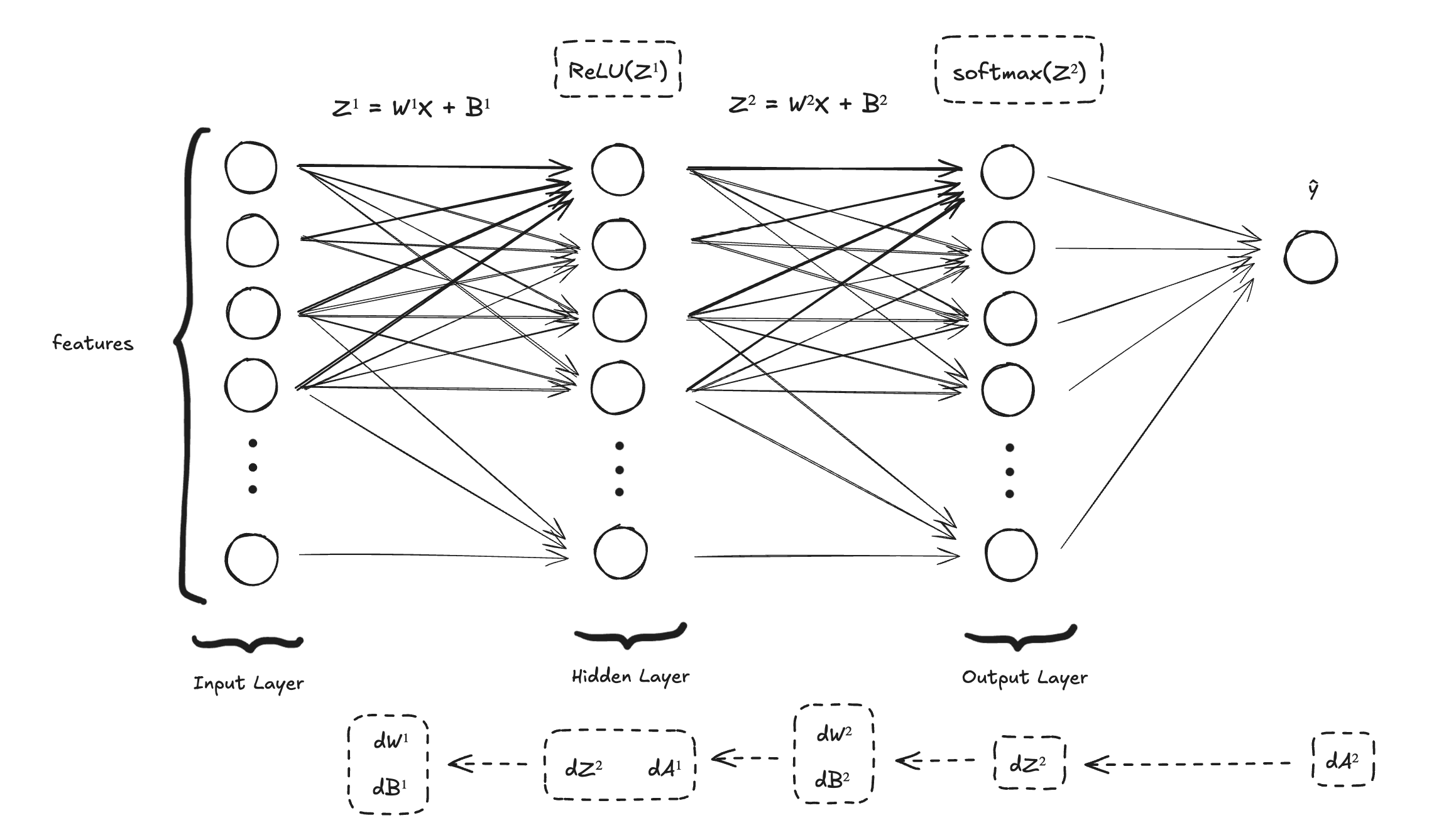
Just a reminder of the neural network we are building: we start with a two-layer neural network, the input layer, the hidden layer, and the output layer.

The shape of the input layer is m = 42,000 and n = 784. We start with 10 neurons (hidden units) in the hidden layer and 10 neurons in the output layer. We use 10 neurons in the output layer because we want to represent all the possible digits (from 0 to 9). The softmax function takes a vector of logits from these 10 neurons and converts it into a probability distribution over the 10 classes, where the sum of probabilities equals 1, making the interpretation straightforward.

Here how it looks like:

The first thing we need to do is import the libraries we are going to use: numpy and pandas

import numpy as np
import pandas as pd

Numpy is used for vectorization and matrices multiplication, and pandas is used to read the MNIST dataset.

Let's now take a closer look at the data

data = pd.read_csv('/kaggle/input/digit-recognizer/train.csv')
m, n = data.shape
m # 42000
n # 785

As I said before, we have 42,000 training examples and 784 pixels (features) in this dataset. It's 785 though because we also have a column for the label (a digit from 0 to 9). We'll use the neural network to create the relationship between these pixels and the given label.

Each pixel has a value between 0 and 255 (0 is black and 255 white — this the numbers for RGB).

Before moving forward to the neural network implementation, we need to build the data that will be trained, tested, and normalized.

np.random.shuffle(data)

number_of_tests = int(m * 0.3)

test_data = data[0:number_of_tests].T
Y_test = test_data[0]
X_test = test_data[1:n]
X_test = X_test / 255.0

train_data = data[number_of_tests:m].T
Y_train = train_data[0]
X_train = train_data[1:n]
X_train = X_train / 255.0

Before splitting the data between training and test data, we shuffle it and use 30% for the test validation and 70% for the training process. After shuffling, we just need to slice the data matrix.

Two other important parts of this process are the division by 255 and the transpose of the data. With the division by 255, we want to normalize the pixels so it will be 0 or 1. For the transpose, this is an important step because to do matrix multiplication, the rows and columns should match perfectly.

To start the neural network implementation, we first need to run the forward pass, but with initialized weights and biases, in this case, ${W^{[1]}}$ , ${W^{[2]}}$ , ${B^{[1]}}$ , and ${B^{[2]}}$ .

Biases can be initialized with zeros but If initializing with weights all zeros, we compute similar functions in backpropagation, in other words, it computes only one hidden unit (all the hidden units are symmetric).

For biases, we zero out all the values in the matrix:

B1 = np.zeros((10, 1))
B2 = np.zeros((10, 1))

For weights, we randomize all values but multiply them by a small number like 0.01.

W1 = np.random.rand(10, 784) * 0.01
W2 = np.random.rand(10, 10) * 0.01

We do it because if the weight values are too large, the activations of the neurons in deeper layers may saturate.

Saturation happens when the input to these activation functions is too large or too small, causing the output to be very close to either 0 or 1 (in the case of sigmoid), or -1 or 1 (in the case of tanh).

This saturation can make the gradients very small (the gradients vanish), which slows down or even stops learning during backpropagation, a problem known as the vanishing gradient problem.

So that's our function

def init_params():
    W1 = np.random.rand(10, 784) * 0.01
    B1 = np.zeros((10, 1))
    W2 = np.random.rand(10, 10) * 0.01
    B2 = np.zeros((10, 1))
    return W1, B1, W2, B2

As I said earlier, we start with 10 neural (hidden units) but we'll expand this and check how much this change improves the neural network for learning about the data.

With everything in place, we can start implementing the first part of the neural network, the forward propagation.

Here's what we need to implement for the forward propagation:

\begin{equation}Z^{[1]} = W^{[1]} X + B^{[1]}\end{equation}

\begin{equation}A^{[1]} = ReLU(Z^{[1]})\end{equation}

\begin{equation}Z^{[2]} = W^{[2]} A^{[1]} + B^{[2]}\end{equation}

\begin{equation}A^{[2]} = softmax(Z^{[2]})\end{equation}

We divide this into two parts, the first layer (hidden layer) and the second layer (output layer).

The first layer will handle the linear combination with the input $X$ and then apply the ReLU activation function.

Z1 = W1.dot(X) + B1
A1 = ReLU(Z1)

The ReLU function is defined by this equation

\begin{equation}f(Z) = max(Z, 0)\end{equation}

It's very simple to implement it:

def ReLU(Z):
    return np.maximum(Z, 0)

The second layer will receive the ${A^{[1]}}$ (the output of the first layer) as an input and apply the softmax activation function to build a probability distribution over the 10 labels (digits).

Z2 = W2.dot(A1) + B2
A2 = softmax(Z2)

The softmax equation is defined like this:

\begin{equation}softmax(x_i) = \frac{e^{x_i}}{sum_{j=1}^{k} e^{x_j}}\end{equation}

Also easy to implement:

def softmax(Z):
    return np.exp(Z) / sum(np.exp(Z))

And we finish the forward propagation. We generate ${Z^{[1]}}$ , ${A^{[1]}}$ , ${Z^{[2]}}$ , and ${A^{[2]}}$ .

def forward_propagation(W1, B1, W2, B2, X):
    Z1 = W1.dot(X) + B1
    A1 = ReLU(Z1)
    Z2 = W2.dot(A1) + B2
    A2 = softmax(Z2)
    return Z1, A1, Z2, A2

A bunch of linear combinations and application of activation functions.

Let's go for the second part now: backward propagation.

The backpropagation needs to calculate the gradients so we can update the weights and biases in each iteration of the algorithm. It will, then, compute ${dW^{[1]}}$ , ${dW^{[2]}}$ , ${dB^{[1]}}$ , and ${dB^{[2]}}$ .

We start from the back. To compute ${dW^{[2]}}$ and ${dB^{[2]}}$ , we need to calculate ${dZ^{[2]}}$ . As we saw earlier, this is how it's calculated:

\begin{equation}dZ^{[2]} = {A}^{[2]} - Y\end{equation}

And it's implemented like this:

dZ2 = A2 - Y

$Y$ is the one hot encoding of $Y$ in this context.

${dW^{[2]}}$ and ${dB^{[2]}}$ will follow the equations:

\begin{equation}dW^{[2]} = \frac{1}{m} \cdot {dZ}^{[2]} \cdot {A^{[1]}}^T\end{equation}

\begin{equation}dB^{[2]} = \frac{1}{m} \cdot \sum_{i=1}^m dZ^{[2]}\end{equation}

Here's the implementation:

dW2 = 1 / m * dZ2.dot(A1.T)
dB2 = 1 / m * np.sum(dZ2)

Now that we have ${dZ^{[2]}}$ , ${dW^{[2]}}$ , and ${dB^{[2]}}$ , we can compute the gradients for the rest of the neural network.

${dZ^{[1]}}$ is calculated like this:

\begin{equation}dZ^{[1]} = {W^{[2]}}^T \cdot {dZ^{[2]}} \cdot g\'(Z^{[1]})\end{equation}

The implementation:

dZ1 = W2.T.dot(dZ2) * derivative_of_ReLU(Z1)

Here we need to compute the derivative of ReLU. As we saw before, the derivative of the ReLU function if ${Z^{[1]}}$ is greater than 0 is 1, otherwise, it will be 0.

def derivative_of_ReLU(Z):
    return Z > 0

This function returns booleans but it will be used to calculate like we do when we multiply any number with 0s and 1s.

Then we have the ${dW^{[1]}}$ and ${dB^{[1]}}$ :

\begin{equation}dW^{[1]} = \frac{1}{m} \cdot dZ^{[1]} \cdot X^T\end{equation}

\begin{equation}dB^{[1]} = \frac{1}{m} \cdot \sum_{i=1}^m dZ^{[1]}\end{equation}

The implementation is similar to the second layer:

dW1 = 1 / m * dZ1.dot(X.T)
dB1 = 1 / m * np.sum(dZ1)

Now we calculated all the gradients and they can be used to update the weights and biases.

Here it's the full backpropagation function:

def backward_propagation(Z1, A1, Z2, A2, W1, W2, X, Y):
    dZ2 = A2 - Y
    dW2 = 1 / m * dZ2.dot(A1.T)
    dB2 = 1 / m * np.sum(dZ2)
    dZ1 = W2.T.dot(dZ2) * derivative_of_ReLU(Z1)
    dW1 = 1 / m * dZ1.dot(X.T)
    dB1 = 1 / m * np.sum(dZ1)
    return dW1, dB1, dW2, dB2

After the backpropagation, we need to use the computed values to update weights and biases.

Here we implement the update_params function:

def update_params(W1, B1, W2, B2, dW1, dB1, dW2, dB2, LR):
    W1 = W1 - LR * dW1
    B1 = B1 - LR * dB1
    W2 = W2 - LR * dW2
    B2 = B2 - LR * dB2
    return W1, B1, W2, B2

To update these parameters, we just need to multiply it by the learning rate LR and subtract it from the previous parameters. The function returns the updated parameters.

The last part of the neural network implementation is putting everything together and calling it a gradient descent algorithm.

def gradient_descent(X, Y, LR, iterations):
    W1, B1, W2, B2 = init_params()
    one_hot_Y = one_hot(Y)

    for i in range(iterations + 1):
        Z1, A1, Z2, A2 = forward_propagation(W1, B1, W2, B2, X)
        dW1, db1, dW2, db2 = backward_propagation(Z1, A1, Z2, A2, W1, W2, X, one_hot_Y)
        W1, B1, W2, B2 = update_params(W1, B1, W2, B2, dW1, db1, dW2, db2, LR)
        result = A2

    print(get_accuracy(get_predictions(result), Y))

    return W1, B1, W2, B2

This function will receive the features (pixels) $X$ , the label $Y$ , a learning rate LR, and the number of iterations we want to do.

It initializes the parameters and repeats the algorithm iterations times. First computing the forward propagation, then the backward propagation, and updates the parameters (weights and biases).

${A^{[2]}}$ is the result (the class probabilities) in each iteration. We store it in a variable result to see how well it's performing.

The algorithm needs to return the weights and biases so we can use them to validate our test dataset. First, we train the model with the test dataset and then use the parameters to validate.

We can also print the result for different iterations so we know that the neural network is learning:

if i % 10 == 0:
    print("Iteration: ", i)
    predictions = get_predictions(A2)
    print(get_accuracy(predictions, Y))

Finished that part, here it's an example of how we run this algorithm:

W1, B1, W2, B2 = gradient_descent(X_train, Y_train, 0.10, 500)

This is for the training dataset and we collect the parameters to be used in the validation phase.

_, _, _, A2 = forward_propagation(W1, B1, W2, B2, X_test)
predictions = get_predictions(A2)
get_accuracy(predictions, Y_test)

Using the learned parameters but now validation with the test dataset, we get the predictions and compute the accuracy.

Running this algorithm with 10 hidden units (neurons), with a learning rate of 0.1, and 500 iterations, the model's accuracy we've got was 85%. Both for the training and the test datasets.

As an exercise, I also tested updating the 10 hidden units with 100 hidden units in the hidden layer and I've got 88.2% accuracy both in the training and test datasets.

To train with 10 neurons, we initialized the parameters like this:

W1 = np.random.rand(10, 784) * 0.01
B1 = np.zeros((10, 1))
W2 = np.random.rand(10, 10) * 0.01
B2 = np.zeros((10, 1))

To update from 10 to 100 units, we just need to scale the initialization:

W1 = np.random.rand(100, 784) * 0.01
B1 = np.zeros((100, 1))
W2 = np.random.rand(10, 100) * 0.01
B2 = np.zeros((10, 1))

In a future post, I want to expand this algorithm and add more layers so we can test if the neural network learns and performs better. In other words, deep neural networks would perform better than shallow neural nets? Let's see in a future experiment.

Resources

Hey! You may like this newsletter if you're enjoying this blog. ❤

✖

Twitter · Github